LASER Scanner

Introduction

This tutorial explains how to use the laser scanner and how to link the sensor data to a specific frame of the tf tree.

• Lines beginning with $ are terminal commands.

  • To open a new terminal → use the shortcut Ctrl + Alt + T.

  • To open a new tab inside an existing terminal → use the shortcut Ctrl + Shift +T.

  • To kill a process in a terminal → use the shortcut Ctrl + C.

• Lines beginning with # indicate the syntax of the commands.

• Code is separated in boxes.

• Code is case sensitive.

---

Starting the LASER Scanner

By launching the Turtlebot3 simulation, the laser scanner is automatically spawned as well:

$ export TURTLEBOT3_MODEL=waffle

$ ros2 launch turtlebot3_gazebo turtlebot3_house.launch.py

Let’s have a closer look inside the launch file to determine, where the laser scanner is executed.

#!/usr/bin/env python3

import os

from ament_index_python.packages import get_package_share_directory
from launch import LaunchDescription
from launch.actions import IncludeLaunchDescription
from launch.launch_description_sources import PythonLaunchDescriptionSource
from launch.substitutions import ThisLaunchFileDir
from launch.actions import ExecuteProcess
from launch.substitutions import LaunchConfiguration

TURTLEBOT3_MODEL = os.environ['TURTLEBOT3_MODEL']


def generate_launch_description():
    use_sim_time = LaunchConfiguration('use_sim_time', default='true')
    world_file_name = 'turtlebot3_houses/' + TURTLEBOT3_MODEL + '.model'
    world = os.path.join(get_package_share_directory('turtlebot3_gazebo'), 'worlds', world_file_name)
    launch_file_dir = os.path.join(get_package_share_directory('turtlebot3_gazebo'), 'launch')

    return LaunchDescription([
        ExecuteProcess(
            cmd=['gazebo', '--verbose', world, '-s', 'libgazebo_ros_init.so'],
            output='screen'),

        IncludeLaunchDescription(
            PythonLaunchDescriptionSource([launch_file_dir, '/robot_state_publisher.launch.py']),
            launch_arguments={'use_sim_time': use_sim_time}.items(),
        ),
    ])

Our Turtlebot3 model is loaded in the following line:

            cmd=['gazebo', '--verbose', world, '-s', 'libgazebo_ros_init.so'],

The variable world includes the world file turtlebot3_houses/waffle.model. This file is located in turtlebot3_gazebo/worlds and includes the following:

<include>
  <pose>-2.0 -0.5 0.01 0.0 0.0 0.0</pose>
  <uri>model://turtlebot3_waffle</uri>
</include>

Remember that we added models from the turtlebot3 package to our Gazebo Model path in the .bashrc file:

export GAZEBO_MODEL_PATH=$GAZEBO_MODEL_PATH:~/turtlebot3_ws/src/turtlebot3/turtlebot3_simulations/turtlebot3_gazebo/models

In that path we find the model.sdf file, which describes the laser scanner:

<link name="base_scan">
  <inertial>
    <pose>-0.052 0 0.111 0 0 0</pose>
    <inertia>
      <ixx>0.001</ixx>
      <ixy>0.000</ixy>
      <ixz>0.000</ixz>
      <iyy>0.001</iyy>
      <iyz>0.000</iyz>
      <izz>0.001</izz>
    </inertia>
    <mass>0.125</mass>
  </inertial>

  <collision name="lidar_sensor_collision">
    <pose>-0.052 0 0.111 0 0 0</pose>
    <geometry>
      <cylinder>
        <radius>0.0508</radius>
        <length>0.055</length>
      </cylinder>
    </geometry>
  </collision>

  <visual name="lidar_sensor_visual">
    <pose>-0.064 0 0.121 0 0 0</pose>
    <geometry>
      <mesh>
        <uri>model://turtlebot3_waffle/meshes/lds.dae</uri>
        <scale>0.001 0.001 0.001</scale>
      </mesh>
    </geometry>
  </visual>

This is just the geometry description, but the model.sdf also includes the physical description of the laser scanner as a plugin:

  <sensor name="hls_lfcd_lds" type="ray">
    <always_on>true</always_on>
    <visualize>true</visualize>
    <pose>-0.064 0 0.121 0 0 0</pose>
    <update_rate>5</update_rate>
    <ray>
      <scan>
        <horizontal>
          <samples>360</samples>
          <resolution>1.000000</resolution>
          <min_angle>0.000000</min_angle>
          <max_angle>6.280000</max_angle>
        </horizontal>
      </scan>
      <range>
        <min>0.120000</min>
        <max>3.5</max>
        <resolution>0.015000</resolution>
      </range>
      <noise>
        <type>gaussian</type>
        <mean>0.0</mean>
        <stddev>0.01</stddev>
      </noise>
    </ray>
    <plugin name="turtlebot3_laserscan" filename="libgazebo_ros_ray_sensor.so">
      <ros>
        <!-- <namespace>/tb3</namespace> -->
        <argument>~/out:=scan</argument>
      </ros>
      <output_type>sensor_msgs/LaserScan</output_type>
      <frame_name>base_scan</frame_name>
    </plugin>
  </sensor>
</link>

Visualization Exercise

Launch the file and visualize the laserscan in Rviz. The laser scan data is currently published with reference to the frame base_scan. This is decribed in the two files from above:

<plugin name="turtlebot3_laserscan" filename="libgazebo_ros_ray_sensor.so">
  <ros>
    <!-- <namespace>/tb3</namespace> -->
    <argument>~/out:=scan</argument>
  </ros>
  <output_type>sensor_msgs/LaserScan</output_type>
  <frame_name>base_scan</frame_name>
</plugin>

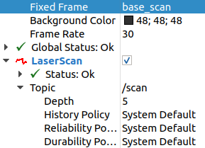
Switch your fixed_frame in RViz to base_scan. Add a laserscan visualization element in RViz, configured to the correct topic for visualization.

Additionally you have to change the QoS policies of the topic so that it matches with the publisher. The best option is to set it to System Default.

Static TF Exercise

Launch turtlebot3_tf.launch.py to publish the static transforms of the turtlebot. Switch the fixed_frame in RViz to base_footprint again. The laserscan data is still available in this frame as the transformation between the frames base_footprint and base_scan is now being broadcasted (see Fig. 1).

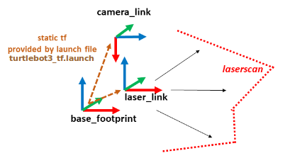
Figure 8 Figure 1. Static TF tree of turtlebot with LASERscan

Dynamic TF Exercise

Launch your node simulated_odom2.py to broadcast the virtual movement of the turtlebot. Switch the fixed_frame in RViz now to odom. Keep in mind that a proper setup of the used TF tree is essential to work with sensor data (see fig. 2).

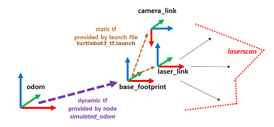
Figure 9 Figure 2. Dynamic TF tree of turtlebot with LASERscan